Life as a Marine Engineer: January 2013

IT Apps - Exercise 9

1 Now it’s your turn to create your own chart! Conduct a short survey of your classmates about a topic of your choice. Some suggestions are:

a) Favourite colour

b) Favourite sport

c) Favourite car

d) Favourite song

e) Least favourite food

2 First create a worksheet then a graph for your survey. You do not necessarily have to do a pie chart. Play around with some options, be creative!

http://mc.tt/d9Kg3NRkKD

IT Apps - Exercise 8

1 The following survey of favourite ice cream flavours will be used for the example.

Chocolate - 6 students

Strawberry - 5 students

Vanilla - 4 students

Rocky Road - 3 students

Peanut Butter Ripple - 2 students

Butter Pecan - 2 students

Neapolitan - 1 student

Black Cherry - 1 student

a) Enter “Ice Cream Survey” in cell A1

b) Enter “Flavour” in cell A2.

c) Enter “Number” in cell B2

d) Enter the flavour names in cells A3 to A10.

e) Enter the corresponding number of students in cells B3 to B10

f) Enter “Total” in cell A11.

2 Now you need to find the total number of the students.

3 Create a pie chart with the title chart “ICE-CREAM SURVEY”

http://mc.tt/71KgJIDNc5

1. Type in the data below into the worksheet
2. Highlight the cells containing the data
3. Click the Insert Tab > Choose 2D Bar Chart
4. The Bar Chart will now appear on the worksheet, edit the chart according to what is shown below.

http://mc.tt/23KgIu6C4D

IT Apps - Exercise 6

In this exercise, you create a worksheet that uses Excel’s Mathematical and statistical functions to generate a value for use in a sweepstakes contest.

Create a worksheet that looks like the one shown below:

Your first step is to populate the worksheet with a list of 10 random integer values between 0 and 100. To do so:

Select: cell A5

Type: =int(rand()*100)

Press: Enter

Copy this from A5 to A14

Random value will appear in each cell.

Then, calculate the average value in D6.

Each person who rents a video will have an opportunity to press F9 key to recalculate the worksheet. If his ‘Average random value’ is greater than the ‘Value to beat’ then he is a winner

4. In cell D8, use the IF functions to informs the participant on how they’ve done. The winner must achieve an average random value that is greater than the specified value to beat. If he wins, cell D8 will displays “Winner!”, otherwise displays “Try Again!”. To do so:

Select: D8

Type: =IF(D6>60, “Winner!”, “Try Again!”)

Press: Enter

In cell range A5 to A14, use conditional formatting fill the cells with blue background if the random value is less than or equal to 60.
In cell D8, also use the Conditional Formatting to fill it with yellow background if the participant wins.
On your own, press the F9 key to test your luck.

http://mc.tt/92KgGSFsqd

IT Apps - Exercise 5

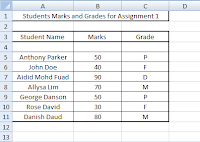
Open a new workbook and develop a spread sheet shown below.
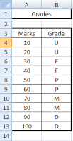
Linkup the two worksheet using VLOOKUP function.
Follow the following steps:

i. In worksheet 2, define the grade table.

ii. Name your table as ‘Grade’.

iii. Now, go to Worksheet 1, and click cell C5

iv. Then Fill in the blank, please refer to the notes on how to do so.

v. Click OK

The Cell C5 will be filling with the grade ‘P’, Use AUTOFILL to copy the formula to the other cells.

Worksheet 1

Worksheet 2

http://mc.tt/a4KgCIv3QD

IT Apps - Exercise 4

Type in the following spreadsheet, and format it to look like the sample below.

1 Type in all text and numbers shown in the spreadsheet below.

2 Format all numbers with appropriate formats.

3 Center the spreadsheet heading 'Total Sales for the Month of November' across the spreadsheet.

4 Format all text as displayed in the sample below, including the rotated text labels.

5 Create formulas to display a total quantity for each fruit.

6 Create formulas to calculate the total sales to each fruit.

7 Apply all borders and shading (color) shown in the sample below, feel free to experiment with your own color schemes.

http://mc.tt/a3KfxmNs7B

IT Apps - Exercise 3

Type in the following spreadsheet, and format it to look like the sample below.

1) Type in all text and numbers shown in the spreadsheet below.
2) Format all numbers as a currency.
3) Center the spreadsheet heading 'Sales and Produce Department' across the spreadsheet.
4) Format all text as displayed in the sample below.
5) Create formulas to display the average sales.
6) Create formulas to display total sales for each salesperson.